Raytracing
A non-rotating black hole is described by:
$$g_{\mu\nu}dx^\mu dx^\nu=-(1-\dfrac{r_s}{r})c^2dt^2+(1-\dfrac{r_s}{r})^{-1}dr^2+r^2d\Omega^2$$
where \(d\Omega^2\) is defined as:
$$d\Omega^2=d\theta^2-\sin^2{\theta}d\varphi^2,\:\:\:\:\:\:r_s=\dfrac{2MG}{c^2}$$
Objects follow the geodesic equation:
$$\dfrac{d^2x^\mu}{ds^2}+\Gamma_{\alpha\beta}^{\mu}\dfrac{dx^\alpha}{ds}\dfrac{dx^\beta}{ds}=0$$
where the Christoffel symbol is given by:
$$\Gamma_{\alpha\beta}^{\mu}=\frac{1}{2}g^{\mu\delta}(\partial_\beta g_{\alpha\delta}+\partial_\alpha g_{\beta\delta}- \partial_\delta g_{\alpha\beta})$$
Due to spherical symmetry one can set:
$$\theta(s):=\dfrac{\pi}{2},\:\:\:\:\:\:\dfrac{d\theta}{ds}(s):=0$$
A light beam is a null geodesic so one finds also:
$$g_{\mu\nu}dx^\mu dx^\nu=0$$

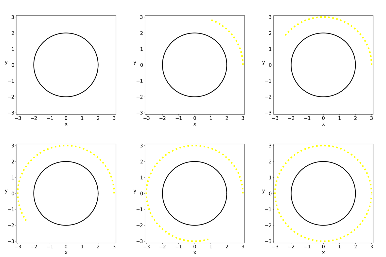
Figure 1: shows the time evolution of a light beam at the innermost bound circular orbit for \(M=1\),\(G=1\) and \(c=1\) which can be found at \(r_{IBCO}=3r_s/2\).
The geodesic equations now become:
$$\dfrac{d^2t}{ds^2}=\dfrac{-2M}{r(r-2M)}\dfrac{dt}{ds}\dfrac{dr}{ds},\:\:\:\:\:\:\:\:\dfrac{d^2\phi}{ds^2}=\dfrac{-2}{r}\dfrac{d\phi}{ds}\dfrac{dr}{ds}$$
$$\dfrac{d^2r}{ds^2}=\dfrac{M}{r(r-2M)}\dfrac{dr}{ds}\dfrac{dr}{ds}-\dfrac{M(r-2M)}{r^3}\dfrac{dt}{ds}\dfrac{dt}{ds}+(r-2M)\dfrac{d\phi}{ds}\dfrac{d\phi}{ds}$$
These equations can be solved numerically via Runge Kutta Methods. The Lagrange function is given by:
$$\mathcal{L}=T-V=-\frac{1}{2}c^2(1-\dfrac{r_s}{r})\dfrac{dt}{ds}\dfrac{dt}{ds}+\frac{1}{2}(\dfrac{1}{1-r_s/r})\dfrac{dr}{ds}\dfrac{dr}{ds}+\frac{1}{2}r^2\dfrac{d\phi}{ds}\dfrac{d\phi}{ds}$$
The Euler Lagrange equation is given by:
$$\dfrac{\partial \mathcal{L}}{d q}-\dfrac{d}{ds}\dfrac{\partial \mathcal{L}}{d \dot{q}}=0$$
one now finds:
$$\dfrac{d}{ds}r^2\dot{\phi}=0\Rightarrow r^2\dot{\phi}=L=constant,\:\:\:\:\:\dfrac{d}{ds}c^2(1-r_s/r)\dot{t}=0\Rightarrow c^2(1-r_s/r)\dot{t}=E=constant$$
Putting these results into \(\mathcal{L}=0\) one finds:
$$-E^2/c^2+\dot{r}^2+(1-r_s/r)\dfrac{L^2}{r^2}=0\Rightarrow V_{eff}=L^2/(2r^2)-L^2r_s/(2r^3)$$
The maximum of \(V_{eff}\) is given by:
$$V_{eff} ’(r)=-L^2/r^3+3L^2r_s/(2r^4)=0\Rightarrow r=r_{IBCO}=\dfrac{3r_s}{2}$$
\(r_{IBCO}\) is the innermost bound circular orbit. For smaller r no circular orbits are possible.
References
[1] https://de.wikipedia.org/wiki/Schwarzschild-Metrik
[2] https://profoundphysics.com/can-light-orbit-a-black-hole-the-physics-explained/
[1] https://de.wikipedia.org/wiki/Schwarzschild-Metrik
[2] https://profoundphysics.com/can-light-orbit-a-black-hole-the-physics-explained/
"""
The code below was written by @author: https://github.com/DianaNtz and is an
implementation of the 2nd order Runge Kutta time integration method for the
geodesic equation of a Schwarzschild black hole.
For more details on the code requirements and licences see
https://github.com/DianaNtz/Raytracing.
"""

#importing libraries
import matplotlib.pyplot as plt
import numpy as np
import matplotlib.animation as animation

#setting up initial values
ntau=10000

M=1

r1n=3.0
r2n=0.0

t1n=0
t2n=0.1

phi1n=0
phi2n=np.sqrt((1-2*M/r1n)/r1n**2*t2n**2)

dtau=(2.0*np.pi/phi2n)/(ntau-1)

taun=0

#setting up functions for time integration
def ft1(t1,t2,r1,r2,phi1,phi2):
              return t2
def fr1(t1,t2,r1,r2,phi1,phi2):
              return r2
def fphi1(t1,t2,r1,r2,phi1,phi2):
              return phi2

def ft2(t1,t2,r1,r2,phi1,phi2):
              return -2*M/(r1*(r1-2*M))*t2*r2

def fr2(t1,t2,r1,r2,phi1,phi2):
              return M/(r1*(r1-2*M))*r2**2-M*(r1-2*M)/r1**3*t2**2+(r1-2*M)*phi2**2

def fphi2(t1,t2,r1,r2,phi1,phi2):

              return -2/r1*phi2*r2

tau=np.zeros(ntau)

r1=np.zeros(ntau)
r2=np.zeros(ntau)

t1=np.zeros(ntau)
t2=np.zeros(ntau)

phi1=np.zeros(ntau)
phi2=np.zeros(ntau)
#loop for time integration Runge Kutta 2
for j in range(0,ntau):
        tau[j]=taun

        r1[j]=r1n
        r2[j]=r2n

        t1[j]=t1n
        t2[j]=t2n

        phi1[j]=phi1n
        phi2[j]=phi2n

        k1r1=dtau*fr1(t1n,t2n,r1n,r2n,phi1n,phi2n)
        k1r2=dtau*fr2(t1n,t2n,r1n,r2n,phi1n,phi2n)

        k1t1=dtau*ft1(t1n,t2n,r1n,r2n,phi1n,phi2n)
        k1t2=dtau*ft2(t1n,t2n,r1n,r2n,phi1n,phi2n)

        k1phi1=dtau*fphi1(t1n,t2n,r1n,r2n,phi1n,phi2n)
        k1phi2=dtau*fphi2(t1n,t2n,r1n,r2n,phi1n,phi2n)


        k2r1=dtau*fr1(t1n+0.5*k1t1,t2n+0.5*k1t2,r1n+0.5*k1r1,r2n+0.5*k1r2,phi1n+0.5*k1phi1,phi2n+0.5*k1phi2)
        k2r2=dtau*fr2(t1n+0.5*k1t1,t2n+0.5*k1t2,r1n+0.5*k1r1,r2n+0.5*k1r2,phi1n+0.5*k1phi1,phi2n+0.5*k1phi2)

        k2t1=dtau*ft1(t1n+0.5*k1t1,t2n+0.5*k1t2,r1n+0.5*k1r1,r2n+0.5*k1r2,phi1n+0.5*k1phi1,phi2n+0.5*k1phi2)
        k2t2=dtau*ft2(t1n+0.5*k1t1,t2n+0.5*k1t2,r1n+0.5*k1r1,r2n+0.5*k1r2,phi1n+0.5*k1phi1,phi2n+0.5*k1phi2)

        k2phi1=dtau*fphi1(t1n+0.5*k1t1,t2n+0.5*k1t2,r1n+0.5*k1r1,r2n+0.5*k1r2,phi1n+0.5*k1phi1,phi2n+0.5*k1phi2)
        k2phi2=dtau*fphi2(t1n+0.5*k1t1,t2n+0.5*k1t2,r1n+0.5*k1r1,r2n+0.5*k1r2,phi1n+0.5*k1phi1,phi2n+0.5*k1phi2)

        t1n=t1n+k2t1
        t2n=t2n+k2t2

        r1n=r1n+k2r1
        r2n=r2n+k2r2

        phi1n=phi1n+k2phi1
        phi2n=phi2n+k2phi2

        taun=taun+dtau


#create animation with matplotlib
x,y=r1*np.cos(phi1),r1*np.sin(phi1)
fig, ax = plt.subplots(figsize=(7,7))
line2 = ax.plot(2*M*np.cos(phi1),2*M*np.sin(phi1),"-",linewidth=3.0,color='k')
line1 = ax.plot(x[0], y[0],color='yellow',linestyle=':',linewidth=6)[0]
ax.set_xlim(-3.1,3.1)
ax.set_ylim(-3.1,3.1)
plt.xlabel("x",fontsize=19)
plt.ylabel(r'y',fontsize=19,rotation=0)
plt.xticks(fontsize= 19)
plt.yticks(fontsize= 19)


i=40
def update(frame):
              # update the line plot:
              line1.set_xdata(x[:frame*i])
              line1.set_ydata(y[:frame*i])
              return (line1, line2)
ani = animation.FuncAnimation(fig=fig, func=update, frames=int(ntau/i), interval=1)
ani.save("animated_IBCO.gif")
plt.show()