Finite Difference Derivatives
The first Finite Difference Derivatives are:
$$u_c'(x)=\dfrac{u(x+h)-u(x-h)}{2h}+\mathcal{O}(h^2),\:\:\:u_f'(x)=\dfrac{u(x+h)-u(x)}{h}+\mathcal{O}(h),\:\:\:u_b'(x)=\dfrac{u(x)-u(x-h)}{h}+\mathcal{O}(h)$$
Where \(u_c'\) is with centered stencils, \(u_f'\) is with forward stencils and \(u_b'\) is with backward stencils.
Let \(u_a\) be the analytical solution to a problem and \(u^{(h)}\) the numerical one with grid resolution \(h\). The convergence test is:
$$
Q_1=\dfrac{|u_a(x)-u^{(h)}(x)|}{|u_a(x)-u^{(h/2)}(x)|}\approx 2^p
$$
Most of the time we do not find an analytical solution so the self convergence test were established:
$$
Q_2=\dfrac{|u^{(h)}(x)-u^{(h/2)}(x)|}{|u^{(h/2)}(x)-u^{(h/4)}(x)|}\approx 2^p
$$
Where \(p\) is the convergence order of the found solution.
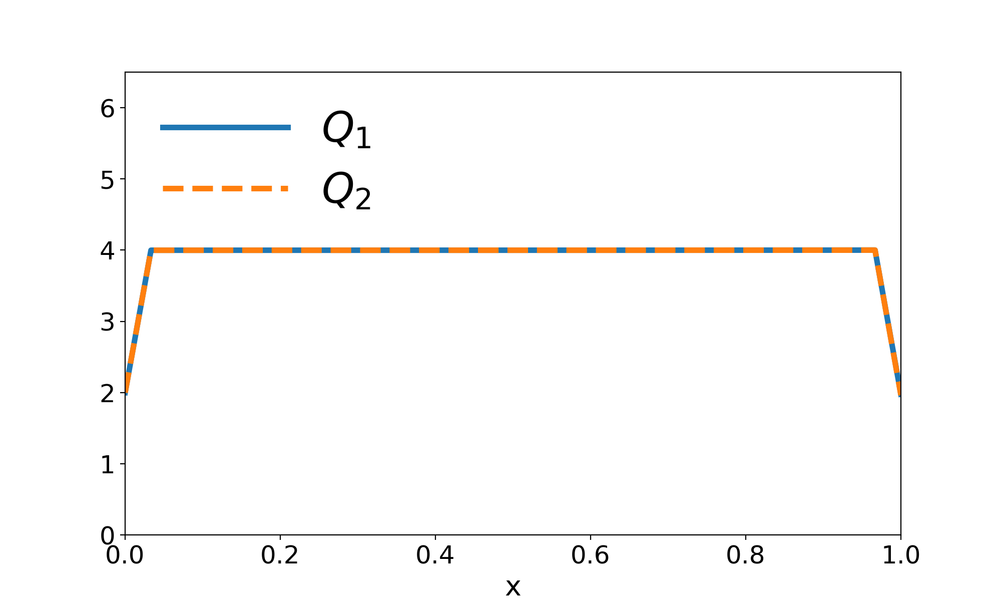
Figure 1: convergence and self convergence tests for \(u(x)=e^{-x^2}\). Forward and backward Derivatives are used for the end points. The convergence order is \(p=1\) for the end points and \(p=2\) for the midpoints.
"""
The code below was written by https://github.com/DianaNtz and
is an implementation of the Finite Difference Derivatives.
"""
#import libraries
import numpy as np
import matplotlib.pyplot as plt

#create a grids with 3 different resolutions.
nx1=30
h1=1/(nx1-1)
x1=np.linspace(0,1,nx1+1)

nx2=nx1*2
h2=1/(nx2-1)
x2=np.linspace(0,1,nx2+1)

nx3=nx2*2
h3=1/(nx3-1)
x3=np.linspace(0,1,nx3+1)

#Finite Difference Derivatives first order
def first(f):
    n=len(f)
    h=1/(n-1)
    fx=np.zeros(n)
    fx[0]=(f[1]-f[0])/h
    fx[n-1]=(f[n-1]-f[n-2])/h
    for i in range(1,n-1):
        fx[i]=(f[i+1]-f[i-1])/(2*h)
    return fx

#test derivatives with example functions
h1f1=np.exp(-x1**2)
h1f1x=first(h1f1)
h1af1x=-np.exp(-x1**2)*2*x1


h2f1=np.exp(-x2**2)
h2f1x=first(h2f1)
h2af1x=-np.exp(-x2**2)*2*x2


h3f1=np.exp(-x3**2)
h3f1x=first(h3f1)
h3af1x=-np.exp(-x3**2)*2*x3

#calculate convergence test
C1=np.zeros(nx1+1)
C2=np.zeros(nx1+1)
for i in range(0,len(x1)):
    C1[i]=np.abs(h1af1x[i]-h1f1x[i])/np.abs(h2af1x[i*2]-h2f1x[i*2])
    C2[i]=(h1f1x[i]-h2f1x[2*i])/(h2f1x[2*i]-h3f1x[4*i])

#plotting results
fig,ax1 = plt.subplots(1, sharex=True, figsize=(10,6))
ax1.plot(x1,C1,linewidth=4.0,label="$Q_1$")
ax1.plot(x1,C2,linestyle='--',linewidth=4.0,label="$Q_2$")
ax1.set_ylim([0,6.5])
ax1.set_xlim([x1[0],x1[-1]])
plt.xlabel("x",fontsize=20)
ax1.legend(loc=2,fontsize=30,handlelength=3,frameon=False)
plt.xticks(fontsize= 18)
plt.yticks(fontsize= 18)
plt.savefig("QConvergencefirst.png",dpi=200)
plt.show()
References
[1] https://en.wikipedia.org/wiki/Finite_difference
[1] https://en.wikipedia.org/wiki/Finite_difference