1D Runge Kutta Method
The Runge Kutta algorithm is a method to solve initial value problems that are specified more precisely as follows:
$$\dfrac{d}{dt}u(t)=f(t,u(t)),\:\:\:\:\:\:\:\:\:\:\:u(t_0)=u_0$$
One reason why the Runge Kutta algorithm is so famous is that the accuracy of the algorithm is increasing with higher orders.
The second order Runge Kutta method is given by:
$$k_1=\Delta t f(t_n,u_n),\:\:\:\:\:\:\:\:\:\:\:k_2=\Delta t f(t_n+\frac{1}{2}\Delta t,u_n+\frac{1}{2}k_1),\:\:\:\:\:\:\:\:\:\:\:u_{n+1}=u_n+k_2$$
The coefficients of the third order are:
$$k_1=\Delta t f(t_n,u_n),\:\:\:\:\:\:\:\:k_2=\Delta t f(t_n+\frac{1}{2}\Delta t,u_n+\frac{1}{2}k_1),\:\:\:\:\:\:\:\:k_3=\Delta t f(t_n+\Delta t,u_n-k_1+2k_2)$$
The next iteration step is:
$$u_{n+1}=u_n+\frac{1}{6}k_1+\frac{2}{3}k_2+\frac{1}{6}k_3$$
The fourth order Runge Kutta methods coefficients are:
$$k_1=\Delta t f(t_n,u_n),\:\:\:\:\:\:\:\:k_2=\Delta t f(t_n+\frac{1}{2}\Delta t,u_n+\frac{1}{2}k_1)$$
$$k_3=\Delta t f(t_n+\frac{1}{2}\Delta t,u_n+\frac{1}{2}k_2),\:\:\:\:\:\:\:\:k_4=\Delta t f(t_n+\Delta t,u_n+k_3)$$
The next iteration step of the fourth order is:
$$u_{n+1}=u_n+\frac{1}{6}k_1+\frac{1}{3}k_2+\frac{1}{3}k_3+\frac{1}{6}k_4$$
In the following we are going to discuss some 1 dimensional examples for the Runge Kutta algorithm although it should be mentioned that this method can also be used for vector valued functions \(u \Rightarrow \vec{u}\) and \(f \Rightarrow \vec{f}\).
\(\:\)
One example for a differential equation is: $$\dfrac{d}{dt}u(t)=-(t-a)u(t),\:\:\:\:\:\:\:\:\:\:\:u(0)=C$$ Its analytical solution is: $$u_a(t)=Ce^{-\frac{1}{2}(t-2a)t}$$ The figure below compares this solution with the one obtained from the Runge Kutta algorithm:
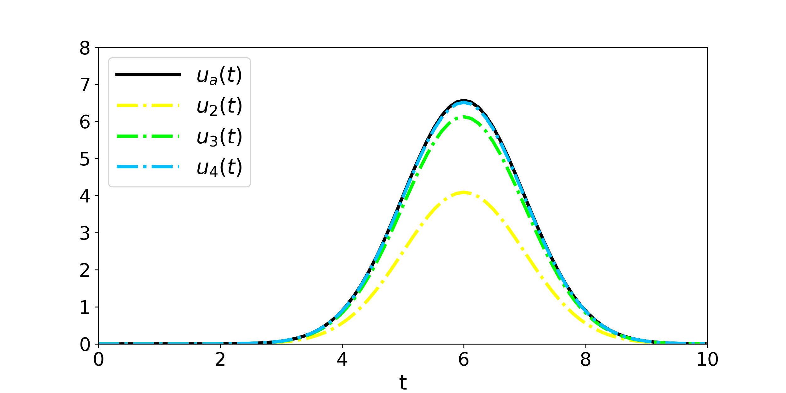
Figure 1: Comparison of the analytical solution \(u_a(t)\) and numerical solution \(u_i(t)\) obtained from the i-th order Runge Kutta method. Notice however that one has set \(t_0=0\:\), \(t_{final}=10\:\), \(dt=0.12\:\), \(C=10^{-7}\:\) and \(a=6\:\).
"""
The code below was written by @author: https://github.com/DianaNtz and is an
implementation of the second, third and fourth order Runge Kutta algorithm.
It solves the differential equation u'=-(t-a)u. For details on requirements
and licences see https://github.com/DianaNtz/Runge-Kutta-Method-Example.
"""
import numpy as np
import matplotlib.pyplot as plt
#some initial values
t0=0
tfinal=10
dt=0.12
steps=int((tfinal-t0)/dt)
u0=0.0000001
a=6
#differential equation function f
def f(t,u):
    return -(t-a)*u
t=np.empty(steps+1, dtype='double')
tn=t0
u2=np.empty(steps+1, dtype='double')
un2=u0
u3=np.empty(steps+1, dtype='double')
un3=u0
u4=np.empty(steps+1, dtype='double')
un4=u0
for i in range(0,steps+1):
    t[i]=tn
    #Runge Kutta second
    u2[i]=un2
    k1=dt*f(tn,un2)
    k2=dt*f(tn+0.5*dt,un2+0.5*k1)
    un2=un2+k2
    #Runge Kutta third
    u3[i]=un3
    k1=dt*f(tn,un3)
    k2=dt*f(tn+0.5*dt,un3+0.5*k1)
    k3=dt*f(tn+dt,un3-k1+2*k2)
    un3=un3+k2*(4/6)+k1*(1/6)+k3*(1/6)
    #Runge Kutta fourth
    u4[i]=un4
    k1=dt*f(tn,un4)
    k2=dt*f(tn+0.5*dt,un4+0.5*k1)
    k3=dt*f(tn+0.5*dt,un4+0.5*k2)
    k4=dt*f(tn+dt,un4+k3)
    un4=un4+k2*(2/6)+k1*(1/6)+k3*(2/6)+k4*(1/6)
    tn=tn+dt
#analytical solution
ua=u0*np.exp(-0.5*(t-a*2)*t)
#plotting analytical vs numerical solutions
ax1 = plt.subplots(1, sharex=True, figsize=(10,5))
plt.plot(t,ua,color='black',linestyle='-',linewidth=3,label="$u_a(t)$")
plt.plot(t,u2,color='yellow',linestyle='-.',linewidth=3,label="$u_2(t)$")
plt.plot(t,u3,color='lime',linestyle='-.',linewidth=3,label = "$u_3(t)$")
plt.plot(t,u4,color='deepskyblue',linestyle='-.',linewidth=3,label = "$u_4(t)$")
plt.xlabel("t",fontsize=19)
plt.ylabel(r' ',fontsize=19,labelpad=20).set_rotation(0)
plt.ylim([0,8])
plt.xlim([t0,tfinal])
plt.xticks(fontsize= 17)
plt.yticks(fontsize= 17)
plt.legend(loc=2,fontsize=19,handlelength=3)
plt.savefig("RungeKutta.png",dpi=120)
plt.show()In a spherical symmetric Newtonian star the gravitational force: $$\vec{F}_{G}=-\frac{G\rho (r)M(r)}{r^2}r^2dr\sin{\theta}d\theta d\varphi\vec{e}_r$$ and pressure force: $$\vec{F}_{P}=-(P(r+dr)-P(r))r^2\sin{\theta}d\theta d\varphi\vec{e}_r$$ are balancing each other out. This can be described mathematically by the Newtonian hydrostatic equation: $$\vec{F}_{G}+\vec{F}_{P}=0\:\:\:\Rightarrow\:\:\:-P'(r)=\frac{G\rho(r)M(r)}{r^2}$$ An analytical solution to the equation above can be found for the constant density case where one assumes: $$\rho (r)=\rho_0\:\:\:\Rightarrow\:\:\:M(r)=\frac{4}{3}\pi r^3\rho_0$$ The Newtonian hydrostatic equation for constant density now reads: $$P'(r)=-\frac{4G\pi}{3}\rho_0^2 r\:\:\:\Rightarrow\:\:\:P(R)-P(r)=-\frac{2G\pi}{3}\rho_0^2(R^2-r^2)$$ where the stars radius \(R\) is defined by \(P(R)=0\). The final result therefore is given by: $$P_a(r)=\frac{2G\pi}{3}\rho_0^2(R^2-r^2)$$ Note that a subscript index \(a\) was added to indicate an analytical solution.
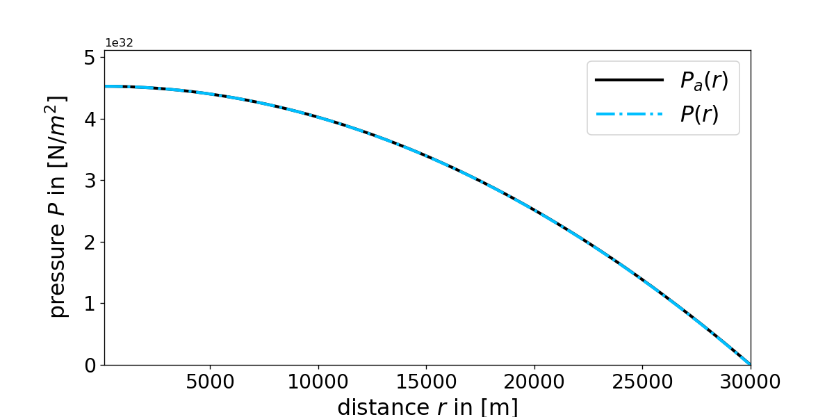
Figure 2: Comparison of the analytical \(P_a (r)\) and numerical solution \(P(r)\) obtained from the fourth order Runge Kutta method for the Newtonian hydrostatic equation with constant density \(\rho_0=6\cdot 10^{16}\:\mathrm{kg/m^3}\) and \(R=30\:\mathrm{km}\).
"""
The code below was written by @author: https://github.com/DianaNtz and is a fourth
order Runge Kutta implementation. It calculates in particular the pressure radius
relation of a spherical symmetric Newtonian star with constant density and compares
it with its analytical solution. For details on requirements and licences see
https://github.com/DianaNtz/Runge-Kutta-Method-Pressure-In-Stars/tree/Newton.
"""
import numpy as np
import matplotlib.pyplot as plt
dr=100 #in m
R=30000 #stars radius in m
Rfinal=R
r0=dr
steps=int(-(r0-Rfinal)/dr)
rho0=6*10**16 #central density of the star in kg/m^3
G=6.67259*10**-11 #gravitational constant in m^3/(kg s^2)
P0=4*np.pi/3*rho0*R**3*G/(2*R)*rho0 #central pressure
def rho(r,rho0,P):
    if(r < =R):
        rho=rho0
    else:
        rho=0
    return rho
def Mass(r,rho0,Parr):
    n=int((r-r0)/dr)
    rint=np.linspace(r0,r,n)
    M=0
    for i in range(0,n):
        M=4*np.pi*rint[i]**2*rho(rint[i],rho0,Parr[i])*dr+M
    return M
def f(r,P,Parr):
    Newton=-G*Mass(r,rho0,Parr)/r**2*rho(r,rho0,P)
    return Newton
P=np.empty(steps+1, dtype='double')
r=np.empty(steps+1, dtype='double')
Pn=P0
rn=r0
#Runge Kutta fourth
for i in range(0,steps+1):
    r[i]=rn
    P[i]=Pn
    k1=dr*f(rn,Pn,P)
    k2=dr*f(rn+0.5*dr,Pn+0.5*k1,P)
    k3=dr*f(rn+0.5*dr,Pn+0.5*k2,P)
    k4=dr*f(rn+dr,Pn+k3,P)
    rn=rn+dr
    Pn=Pn+k2*(2/6)+k1*(1/6)+k3*(2/6)+k4*(1/6)
#analytical solution for constant density star
Pa= 4*np.pi/3*rho0*R**3*G/(2*R)*rho0*(1-(r/R)**2)
ax1 = plt.subplots(1, sharex=True, figsize=(10,5))
plt.plot(r,Pa,color='black',linestyle='-',linewidth=2.5,label = "$P_a(r)$ ")
plt.plot(r,P,color='deepskyblue',linestyle='-.',linewidth=2.5,label="$P(r)$ ")
plt.xlabel("distance $r$ in [m]",fontsize=19)
plt.ylabel(r'pressure $P$ in [N/$m^2$]',fontsize=19,labelpad=10)
plt.xlim([r0,Rfinal])
plt.ylim([0,P0+P0*0.13])
plt.xticks(fontsize= 17)
plt.yticks(fontsize= 17)
plt.legend(loc=1,fontsize=19,handlelength=3)
plt.savefig("Newton.png",dpi=120)
plt.show()
Now let us take a look on a more complicated example than the example above with constant density. Starting from:
$$-P'(r)=\frac{G\rho(r)M(r)}{r^2}$$
and assuming a polytropic equation of state:
$$P=k\rho^{\gamma},\:\:\:\gamma:=\frac{n+1}{n}$$
one obtains:
$$-\frac{kr^2\gamma\rho^{\gamma-1}\rho'}{G\rho}=M$$
derivating this once more brings us to:
$$-\frac{k\gamma}{G(\gamma-1)}(r^2(\rho^{\gamma-1})')'=4\pi r^2\rho,\:\:\:\mathrm{for}\:\gamma\neq 1$$
and
$$\Big(-\frac{kr^2}{G}\Big(\frac{\rho'}{\rho}\Big)\Big)'=4\pi r^2\rho,\:\:\:\mathrm{for}\:\gamma= 1$$
dividing by \(\rho (0)\) one finds:
$$-\frac{k\gamma\rho(0)^{\gamma-2}}{4\pi G(\gamma-1)}\frac{1}{r^2}\frac{d}{dr}\Big(r^2\frac{d}{dr}\Big(\frac{\rho}{\rho(0)}\Big)^{\gamma-1}\Big)=\frac{\rho}{\rho(0)}$$
Now let:
$$\Theta (r):=\Big(\frac{\rho(r)}{\rho(0)}\Big)^{\gamma-1}$$
The equation above becomes therefore:
$$-\frac{k\gamma\rho(0)^{\gamma-2}}{4\pi G(\gamma-1)}\frac{1}{r^2}\frac{d}{dr}\Big(r^2\frac{d}{dr}\Theta\Big)=\Theta^n$$
If one defines:
$$\xi:=\Big(\frac{4\pi G(\gamma-1)}{k\gamma}\Big)^{1/2}\rho (0)^{(2-\gamma)/2}r$$
this results in the well known Lane Emden equation:
$$\frac{1}{\xi^2}\frac{d}{d\xi}\Big(\xi^2\frac{d}{d\xi}\Theta\Big)+\Theta^n=0$$
for \(n=1\) there exists even an analytical solution:
$$\Theta (\xi)=\frac{\sin{\xi}}{\xi}$$
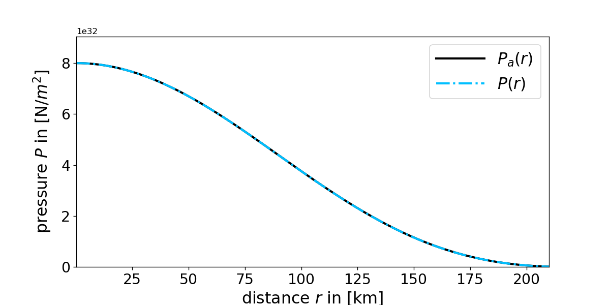
Figure 3: Comparison of the analytical \(P_a (r)\) and numerical solution \(P(r)\) obtained from the fourth order Runge Kutta method for the Newtonian hydrostatic equation with polytropic equation of state n=1. Note however that one has set the central density \(\rho_0=2\cdot 10^{16}\:\mathrm{kg/m^3}\) and \(k=2\:\mathrm{m^5/(kg\:s^2)}\)
"""
The code below was written by @author: https://github.com/DianaNtz and is a fourth order
Runge Kutta implementation. It solves in particular the equation of hydrostatic
equilibrium for a spherical symmetric star with polytropic equation of state and compares
it with the analytical solution for polytropic index n=1. For details on requirements and
licences see https://github.com/DianaNtz/Runge-Kutta-Method-Pressure-In-Stars/tree/Lane.
"""
import numpy as np
import matplotlib.pyplot as plt
dr=100 #in m
R=210000 #in m
Rfinal=R
r0=dr
steps=int(-(r0-Rfinal)/dr)
rho0=2*10**16 #central density of the star in kg/m^3
G=6.67259*10**-11 #gravitational constant in m^3/(kg s^2)
n=1 #dimensionless
k=2 #m^5/kg/s^2 for n=1
P0=k*rho0**(1+1/n) #central pressure
def rho(r,rho0,P):
    return ((1/k)*P)**(n/(n+1))
def Mass(r,rho0,Parr):
    n=int((r-r0)/dr)
    rint=np.linspace(r0,r,n)
    M=0
    for i in range(0,n):
        M=4*np.pi*rint[i]**2*rho(rint[i],rho0,Parr[i])*dr+M
    return M
def f(r,P,Parr):
    Lane=-G/r**2*Mass(r,rho0,Parr)*rho(r, rho0, P)
    return Lane
P=np.empty(steps+1, dtype='double')
r=np.empty(steps+1, dtype='double')
Pn=P0
rn=r0
#Runge Kutta fourth
for i in range(0,steps+1):
    r[i]=rn
    P[i]=Pn
    k1=dr*f(rn,Pn,P)
    k2=dr*f(rn+0.5*dr,Pn+0.5*k1,P)
    k3=dr*f(rn+0.5*dr,Pn+0.5*k2,P)
    k4=dr*f(rn+dr,Pn+k3,P)
    rn=rn+dr
    Pn=Pn+k2*(2/6)+k1*(1/6)+k3*(2/6)+k4*(1/6)
#analytical solution of the Lane Emden equation for n=1
gamma=1/n+1
zeta=np.sqrt(4*np.pi*G*(gamma-1)/(k*gamma))*r*rho0**((2-gamma)/2)
theta=np.sin(zeta)/zeta
rhoa=theta**n*rho0
Pa=k*rhoa**gamma
ax1 = plt.subplots(1, sharex=True, figsize=(10,5))
plt.plot(r/1000,Pa,color='black',linestyle='-',linewidth=2.5,label = "$P_a(r)$ ")
plt.plot(r/1000,P,color='deepskyblue',linestyle='-.',linewidth=2.5,label="$P(r)$ ")
plt.xlabel("distance $r$ in [km]",fontsize=19)
plt.ylabel(r'pressure $P$ in [N/$m^2$]',fontsize=19,labelpad=10)
plt.xlim([r0/1000,Rfinal/1000])
plt.ylim([0,P0+P0*0.13])
plt.xticks(fontsize= 17)
plt.yticks(fontsize= 17)
plt.legend(loc=1,fontsize=19,handlelength=3)
plt.savefig("Lane.png",dpi=120)
plt.show()
Now let us take a look at a general static spherical symmetric metric:
$$g_{\mu\nu}dx^\mu dx^\nu=e^{\eta (r)}c^2dt^2-e^{\xi (r)}dr^2-r^2d\theta^2-r^2\sin^2{\theta}d\varphi^2$$
The stress energy tensor for a perfect fluid is diagonal that means
$$T_0^0=\rho (r)c^2,\:\:\:\:T_i^j=-P(r)\delta_i^j$$
The Einstein field equations are given by:
$$G_{\mu\nu}=\frac{8\pi G}{c^4}T_{\mu\nu}$$
From the \(G_{00}\) component one finds:
$$\frac{8\pi G}{c^4}\rho (r)c^2e^{\eta (r)}=\frac{e^{\eta (r)}}{r^2}(1-\frac{d}{dr}re^{-\xi (r)})\:\:\:\Rightarrow\:\:e^{-\xi (r)}=1-\frac{2GM(r)}{rc^2}$$
The \(G_{11}\) component leads us to:
$$-\frac{8\pi G}{c^4}P(r)e^{\xi (r)}=\frac{-r\eta'(r)+e^{\xi (r)}-1}{r^2}$$
Plugging in the result for \(e^{\xi (r)}\) one finds:
$$\frac{d\eta}{dr}=\frac{1}{r}\Big(1-\frac{2GM(r)}{c^2r}\Big)^{-1}\Big(\frac{8\pi G}{c^4}P(r)r^2+\frac{2GM(r)}{c^2r}\Big)$$
from \(\nabla_\mu T_\nu^\mu=0\) and \(\partial _t\rho=\partial_tP=0\) one finds:
$$\nabla_\mu T_1^\mu=-\frac{dP}{dr}-\frac{1}{2}(P+\rho c^2)\frac{d\eta}{dr}=0\:\:\:\Rightarrow\:\:-P'(r)=\frac{1}{2}(P(r)+\rho (r)c^2)\eta'(r)$$
If one plugs in \(\eta'(r)\) this results in the Tolman Oppenheimer Volkoff equation:
$$-P'(r)=G\frac{M(r)+4\pi r^3P(r)/c^2}{r^2(1-\frac{2GM(r)}{c^2r})}(\rho(r)+P(r)/c^2)$$
An example where the above equation can be solved analytically is for constant density:
$$\rho (r)=\rho_0\:\:\:\Rightarrow\:\:\:M(r)=\frac{4}{3}\pi r^3\rho_0$$
The above equation now reads:
$$-P'(r)=G\frac{4}{3}\pi r\frac{\rho_0+3 P(r)/c^2}{(1-\frac{8G\pi\rho_0}{3c^2}r^2)}(\rho_0+P(r)/c^2)$$
multiplying by \(-2\rho_0 c^2\) it becomes:
$$2\rho_0 c^2P'(r)=-\frac{8G\pi\rho_0}{3c^2} r\frac{\rho_0c^2+3 P(r)}{(1-\frac{8G\pi\rho_0}{3c^2}r^2)}(\rho_0c^2+P(r))$$
in differential form this reads:
$$\frac{2\rho_0 c^2}{(\rho_0c^2+3 P(r))(\rho_0c^2+P(r))}dP=-\frac{8G\pi\rho_0}{3c^2}\frac{r}{(1-\frac{8G\pi\rho_0}{3c^2}r^2)}dr$$
for simplicity one defines the constant \(d\) as:
$$\frac{1}{d^2}:=\frac{8G\pi\rho_0}{3c^2}=\frac{2G\frac{4}{3}\pi R^3\rho_0}{c^2R^3}=r_s/R^3$$
Integrating from \(r'\) to \(R\) one obtains for the right hand side:
$$-\frac{1}{d^2}\int_{r'}^R\frac{r}{1-\frac{r^2}{d^2}}dr=-\frac{1}{2}\int_{r'^2/d^2}^{R^2/d^2}\frac{1}{1-u}du=\frac{1}{2}\ln{\Big(\frac{1-R^2/d^2}{1-r'^2/d^2}\Big)}$$
For the left hand side one does a partial fraction decomposition:
$$\frac{A}{\rho_0c^2+3 P(r)}+\frac{B}{\rho_0c^2+P(r)}=\frac{2\rho_0 c^2}{(\rho_0c^2+3 P(r))(\rho_0c^2+P(r))}\:\:\:\Rightarrow\:\:\:B=-1,\:\:A=3$$
So one obtains
$$\int_{P(r')}^{P(R)}\frac{1}{\rho_0 c^2/3+P(r)}-\frac{1}{\rho_0c^2+P(r)}dP=\Big[\ln{\Big(\frac{\rho_0c^2/3+P(r)}{P(r)+\rho_0c^2}\Big)}\Big]_{P(r')}^{P(R)}$$
Note that for the star radius \(R\) one finds \(P(R)=0\), so one obtains:
$$\ln{\Big(\frac{\rho_0c^2/3}{\rho_0c^2/3+P(r')}\frac{\rho_0c^2+P(r')}{\rho_0c^2}\Big)}=\ln{\Big(\frac{\sqrt{1-R^2/d^2}}{\sqrt{1-r'^2/d^2}}\Big)}$$
This leads us to:
$$\frac{\rho_0c^2+P(r')}{\rho_0c^2+3P(r')}=\frac{\sqrt{1-r_s/R}}{\sqrt{1-r'^2r_s/R^3}}$$
which can also be written as:
$$P(r')(1-3\frac{\sqrt{1-r_s/R}}{\sqrt{1-r'^2r_s/R^3}})=(\frac{\sqrt{1-r_s/R}}{\sqrt{1-r'^2r_s/R^3}}-1)\rho_0c^2$$
This leads us to the final result:
$$P_a(r)=\rho_0c^2\frac{\sqrt{1-r^2r_s/R^3}-\sqrt{1-r_s/R}}{3\sqrt{1-r_s/R}-\sqrt{1-r^2r_s/R^3}}$$
Note that a subscript index \(a\) was added to indicate an analytical solution. Note further that \(r'\) was substituted by \(r\).
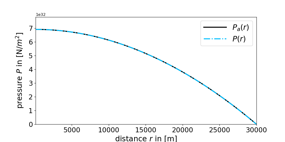
Figure 4: Comparison of the analytical \(P_a (r)\) and numerical solution \(P(r)\) obtained from the fourth order Runge Kutta method for the Tolman Oppenheimer Volkoff equation with constant density \(\rho_0=6\cdot 10^{16}\:\mathrm{kg/m^3}\).
The above equations now lead us to \(\xi_a(r)=\ln{((1-r^2r_s/R^3)^{-1})}\).
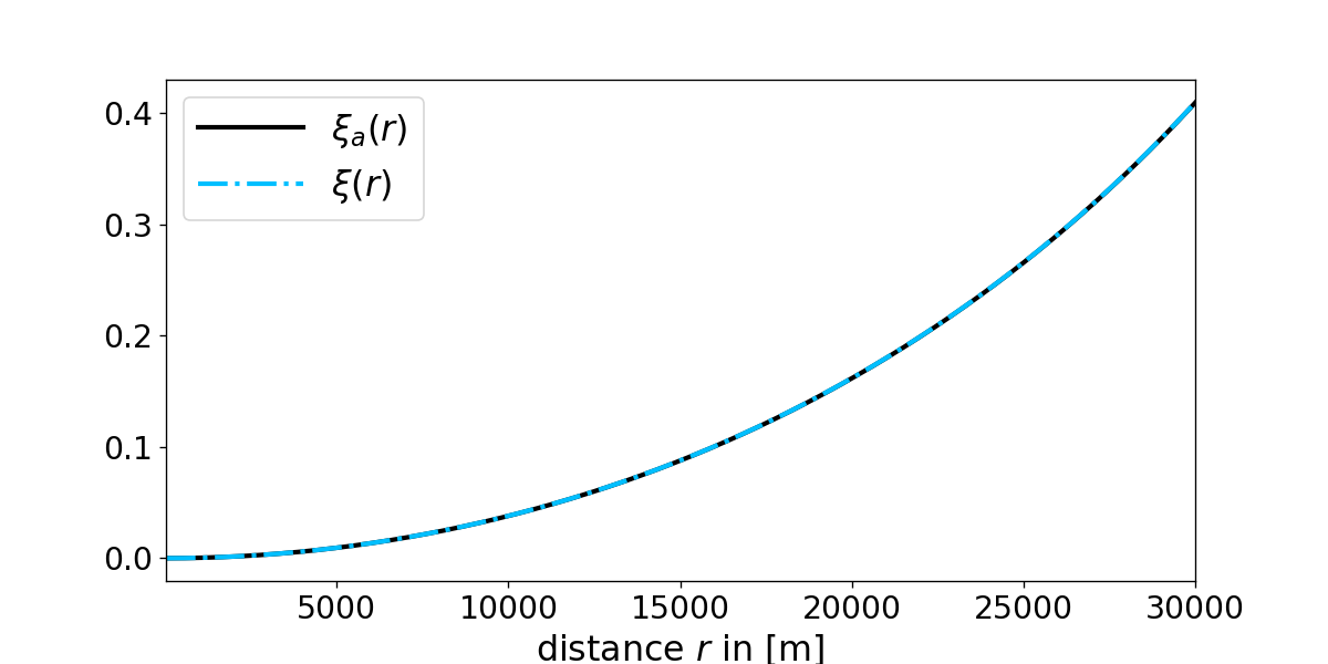
Figure 4: Comparison of the analytical \(\xi_a (r)\) and numerical solution \(\xi(r)\) obtained from the fourth order Runge
Kutta method for the Tolman Oppenheimer Volkoff equation with constant density \(\rho_0=6\cdot 10^{16}\:\mathrm{kg/m^3}\).
Furthermore we obtain \(\eta_a(r)=\ln{\bigg(\frac{1}{4}\Big(3\sqrt{1-r_s/R}-\sqrt{1-r^2r_s/R^3}\Big)^2\bigg)}\).
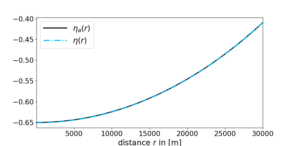
Figure 4: Comparison of the analytical \(\eta_a (r)\) and numerical solution \(\eta(r)\) obtained from the fourth order Runge
Kutta method for the Tolman Oppenheimer Volkoff equation with constant density \(\rho_0=6\cdot 10^{16}\:\mathrm{kg/m^3}\).
"""
The code below was written by @author: https://github.com/DianaNtz and is a fourth
order Runge Kutta implementation. It solves in particular the Tolman Oppenheimer
Volkoff equation (TOV) for a spherical symmetric star with constant density and
compares it with its analytical solution. For details on requirements and licences
see https://github.com/DianaNtz/Runge-Kutta-Method-Pressure-In-Stars/tree/TOV.
"""
import numpy as np
import matplotlib.pyplot as plt
dr=25 #in m
R=30000 #star radius in m
Rfinal=R
r0=dr
steps=int(-(r0-Rfinal)/dr)
c=299792458 #speed of light in m/s
rho0=6*10**16 #central density of the star in kg/m^3
G=6.67259*10**-11 #gravitational constant in m^3/(kg s^2)
rs=2*G/c**2*(4*np.pi/3*rho0*R**3) #schwarzschild radius
P0=rho0*c**2*(1-np.sqrt(1-rs/R))/(3*np.sqrt(1-rs/R)-1) #central pressure
def rho(r,rho0,P):
    if(r<=R):
        rho=rho0
    else:
        rho=0
    return rho
def Mass(r,rho0,Parr):
    n=int((r-r0)/dr)
    rint=np.linspace(r0,r,n)
    M=0
    for i in range(0,n):
        M=4*np.pi*rint[i]**2*rho(rint[i],rho0,Parr[i])*dr+M
    return M
def f(r,P,Parr):
    TOV=-G*(Mass(r,rho0,Parr)+4*np.pi*r**3*P/c**2)/(r**2*(1-2*G*Mass(r,rho0,Parr)
    /(r*c**2)))*(rho(r,rho0,P)+P/c**2)
    return TOV
P=np.empty(steps+1, dtype='double')
M=np.empty(steps+1, dtype='double')
xi=np.empty(steps+1, dtype='double')
deta=np.empty(steps+1, dtype='double')
eta=np.empty(steps+1, dtype='double')
r=np.empty(steps+1, dtype='double')
Pn=P0
rn=r0
#Runge Kutta fourth
for i in range(0,steps+1):
    r[i]=rn
    P[i]=Pn
    M[i]=Mass(rn,rho0,P)
    deta[i]=-2*f(rn,Pn,P)/(P[i]+rho(r[i],rho0,P[i])*c**2)
    k1=dr*f(rn,Pn,P)
    k2=dr*f(rn+0.5*dr,Pn+0.5*k1,P)
    k3=dr*f(rn+0.5*dr,Pn+0.5*k2,P)
    k4=dr*f(rn+dr,Pn+k3,P)
    rn=rn+dr
    Pn=Pn+k2*(2/6)+k1*(1/6)+k3*(2/6)+k4*(1/6)
dn=-np.log(1/(1-2*G*M[-1]/(R*c**2)))
for i in range(steps,-1,-1):
    dn=dn-dr*deta[i]
    eta[i]=dn
xi=np.log(1/(1-2*G*M/(r*c**2)))
#analytical solution for constant density star
Pa=rho0*c**2*(np.sqrt(1-r**2*rs/R**3)
-np.sqrt(1-rs/R))/(3*np.sqrt(1-rs/R)-np.sqrt(1-r**2*rs/R**3))
xia=np.log(1/(1-rs*r**2/R**3))
etaa=np.log(0.25*(3*np.sqrt(1-rs/R)-np.sqrt(1-r**2*rs/R**3))**2)
ax1 = plt.subplots(1, sharex=True, figsize=(10,5))
plt.plot(r,Pa,color='black',linestyle='-',linewidth=2.5,label = "$P_a(r)$ ")
plt.plot(r,P,color='deepskyblue',linestyle='-.',linewidth=2.5,label="$P(r)$ ")
plt.xlabel("distance $r$ in [m]",fontsize=19)
plt.ylabel(r'pressure $P$ in [N/$m^2$]',fontsize=19,labelpad=10)
plt.xlim([r0,Rfinal])
plt.ylim([0,P0+P0*0.13])
plt.xticks(fontsize= 17)
plt.yticks(fontsize= 17)
plt.legend(loc=1,fontsize=19,handlelength=3)
plt.savefig("TOV.png",dpi=120)
plt.show()
ax1 = plt.subplots(1, sharex=True, figsize=(10,5))
plt.plot(r,xia,color='black',linestyle='-',linewidth=2.5,label = "$ξ_a(r)$ ")
plt.plot(r,xi,color='deepskyblue',linestyle='-.',linewidth=2.5,label="$ξ(r)$ ")
plt.xlabel("distance $r$ in [m]",fontsize=19)
plt.xlim([r0,Rfinal])
plt.xticks(fontsize= 17)
plt.yticks(fontsize= 17)
plt.legend(loc=2,fontsize=19,handlelength=3)
plt.savefig("xi.png",dpi=120)
plt.show()
ax1 = plt.subplots(1, sharex=True, figsize=(10,5))
plt.plot(r,etaa,color='black',linestyle='-',linewidth=2.5,label = "$η_a(r)$ ")
plt.plot(r,eta,color='deepskyblue',linestyle='-.',linewidth=2.5,label="$η(r)$ ")
plt.xlabel("distance $r$ in [m]",fontsize=19)
plt.xlim([r0,Rfinal])
plt.xticks(fontsize= 17)
plt.yticks(fontsize= 17)
plt.legend(loc=2,fontsize=19,handlelength=3)
plt.savefig("eta.png",dpi=120)
plt.show()