Spectral Method PDE

The Poisson equation is given by: $$\Delta u=f\:\:\:\in\Omega\:\:\: and \:\:\:u(z)=0 \:\:\:\forall\: z\in\partial\Omega$$ Kronecker product of two matrix $A$ and $B$ is given by: $$A\otimes B=\begin{pmatrix} a_{11}B&...&a_{1n}B\\ \vdots&\vdots&\vdots\\ a_{m1}B&...&a_{mn}B\\ \end{pmatrix}$$ In two dimensions the spectral operator can be constructed with the Kronecker product as following: $$\Delta=I_y\otimes D_x+D_y\otimes I_x$$ The function $f$ can be written in: $$f=f(y)\otimes f(x)$$ This is equivalent to write the two dimensional object as one dimensional in the following way: $$f_{j,i}\Rightarrow f_{i+N_x j}$$

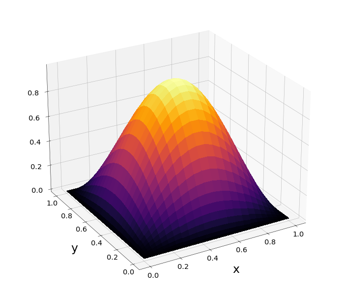
Figure 1: $\Omega=[0,1]\times[0,1]$ and $f=2\pi^2\sin{(\pi x)}\sin{(\pi y)}$

References
[1] https://www.sciencedirect.com/science/article/pii/S0307904X12005938

To get the code go to my GitHub repository PDE

View Code

"""The code below was written by @author: https://github.com/DianaNtz and
solves the Poisson equation via spectral methods. """
import numpy as np
import matplotlib.pyplot as plt
from matplotlib import cm

#create grid
def Cheb_grid_and_D(xmin,xmax,Nx):
     x=np.zeros(Nx)
     cx=(xmax-xmin)/2
     dx=(xmax+xmin)/2
     for j in range(0,Nx):
         x[j]=-np.cos(j*np.pi/(Nx-1))*cx+dx
     Dx=np.zeros((Nx,Nx))
     Dx[0][0]=-(2*(Nx-1)**2+1)/6
     Dx[Nx-1][Nx-1]=(2*(Nx-1)**2+1)/6
     for i in range(0,Nx):
         if(i==0 or i==Nx-1):
             ci=2
         else:
             ci=1
         for j in range(0,Nx):
             if(j==0 or j==Nx-1):
                 cj=2
             else:
                 cj=1
             if(i==j and i!=0 and i!=Nx-1):
                Dx[i][i]=-((x[i]-dx)/cx)/(1-((x[i]-dx)/cx)**2)*0.5
             if(i!=j):
                Dx[i][j]=ci/cj*(-1)**(i+j)/(x[i]/cx-x[j]/cx)

     Dx=Dx/cx
     return x,Dx,np.dot(Dx,Dx)

#Initial values
Nx=30
Ny=40

xmin=0
xmax=1.0

ymax=1.0
ymin=0.0


y,Dy,D2y=Cheb_grid_and_D(ymin,ymax,Ny)
x,Dx,D2x=Cheb_grid_and_D(xmin,xmax,Nx)

d2x=np.kron(np.identity((Ny)),D2x)
d2y=np.kron(D2y,np.identity((Nx)))

f=np.zeros(Ny*Nx)


for j in range(0,Ny):
          for i in range(0,Nx):
                  f[i+j*Nx]=-2*np.pi**2*np.sin(np.pi*y[j])*np.sin(np.pi*x[i])
#create Laplace operator
L=d2y+d2x
#setting boundaries
bound=np.kron(np.identity((Ny)),np.identity((Nx)))
b=f
for j in range(0,Ny):
        for i in range(0,Nx):
            if(i==0):
               b[i+j*Nx]=0
            if(i==Nx-1):
               b[i+j*Nx]=0
            if(j==Ny-1):
               b[i+j*Nx]=0
            if(j==0):
               b[i+j*Nx]=0



for k in range(0,Ny*Nx):
        if(k%Nx==0):
           #z bei 0
           L[k]=bound[k]
        if(k < Nx ):
           L[k]=bound[k]
           #rho bei 0
        if(k%Nx==Nx-1):
           L[k]=bound[k]
           #z bei Nz
        if(k>=Ny*Nx-Nx):
           L[k]=bound[k]
           #rho bei Nrho
#solve linear system
solution=np.linalg.solve(L,b)
print(np.linalg.matrix_rank(L,tol=0.000000000000001))
print(Ny*Nx)

so=solution.reshape(Ny,Nx)

#plotting results
xx,yy= np.meshgrid(x, y)
fig = plt.figure(figsize=(14,12))
axx = plt.axes(projection='3d')
axx.plot_surface(xx, yy, so,cmap=cm.inferno,antialiased=False)
axx.view_init(azim=240,elev=25)
axx.set_xlabel('x', labelpad=30,fontsize=34)
axx.set_ylabel("y",labelpad=30,fontsize=34)
axx.zaxis.set_tick_params(labelsize=21,pad=18)
axx.yaxis.set_tick_params(labelsize=21)
axx.xaxis.set_tick_params(labelsize=21)
fig.subplots_adjust(left=0, right=1, bottom=0, top=1)
filename ="PDE.png"
plt.savefig(filename,dpi=50)
plt.show()

Spectral Method PDE

Figure 1: \(\Omega=[0,1]\times[0,1]\) and \(f=2\pi^2\sin{(\pi x)}\sin{(\pi y)}\)